CoT Information: Improved Sample Complexity under Chain-of-Thought Supervision

Learning to Think: The Chain-of-Thought Advantage↩

Chain-of-thought (CoT) training has quickly become central to the reasoning breakthroughs of large language models. By supervising models not only on final answers but also on the intermediate reasoning steps, CoT training teaches them how to think, not just what to predict. This shift has enabled LLMs to tackle problems that require multi-step reasoning—tasks where conventional models trained end-to-end often fail.

We can see this difference in action when both models attempt the same problem.

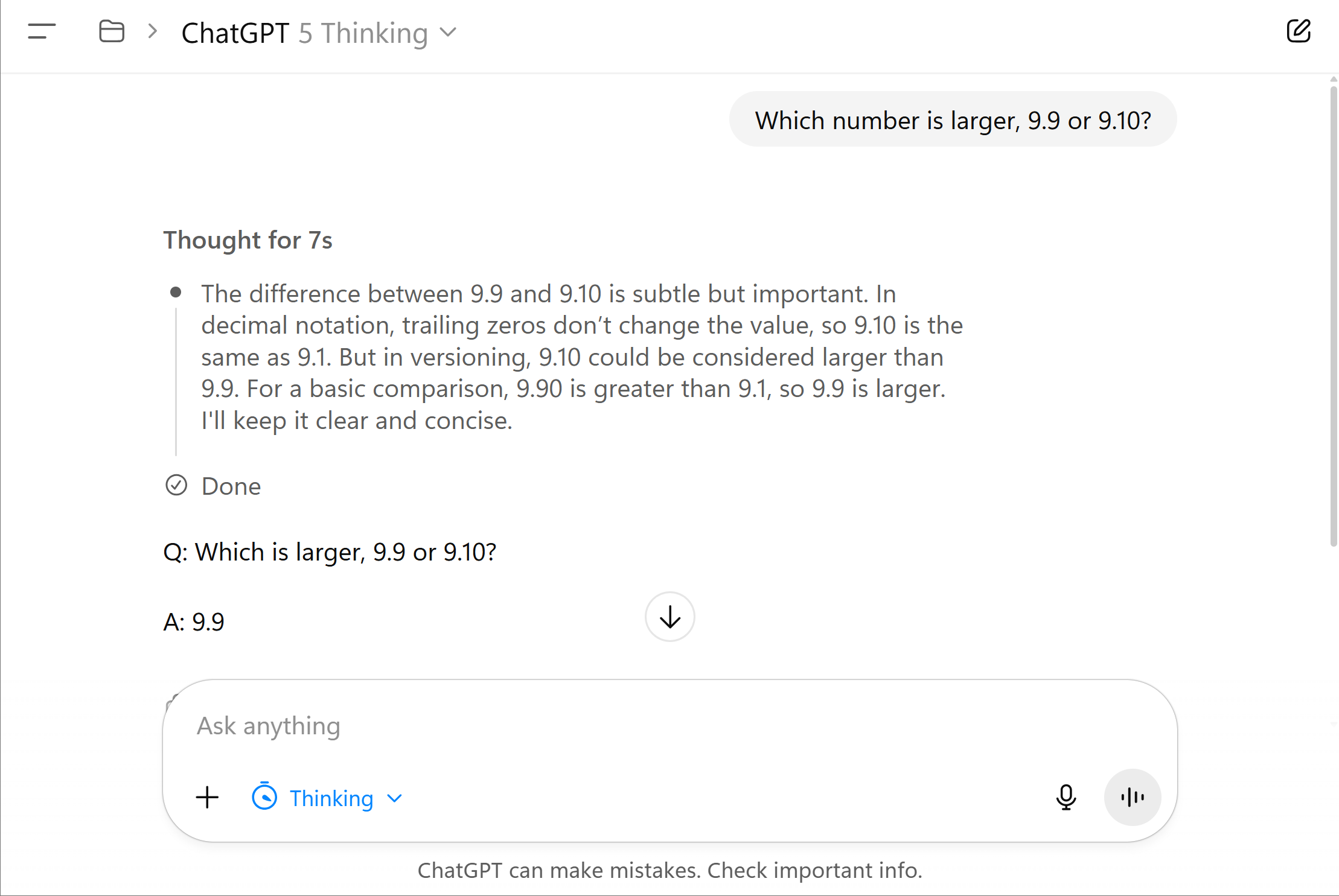
Question. Which number is larger, 9.9 or 9.10?

Question. A forest has 1000 trees. Each year, loggers cut down half of the trees remaining at the start of the year. In the same year, conservationists plant 100 new trees at the end of the year. After this process repeats for two years, how many trees are in the forest?

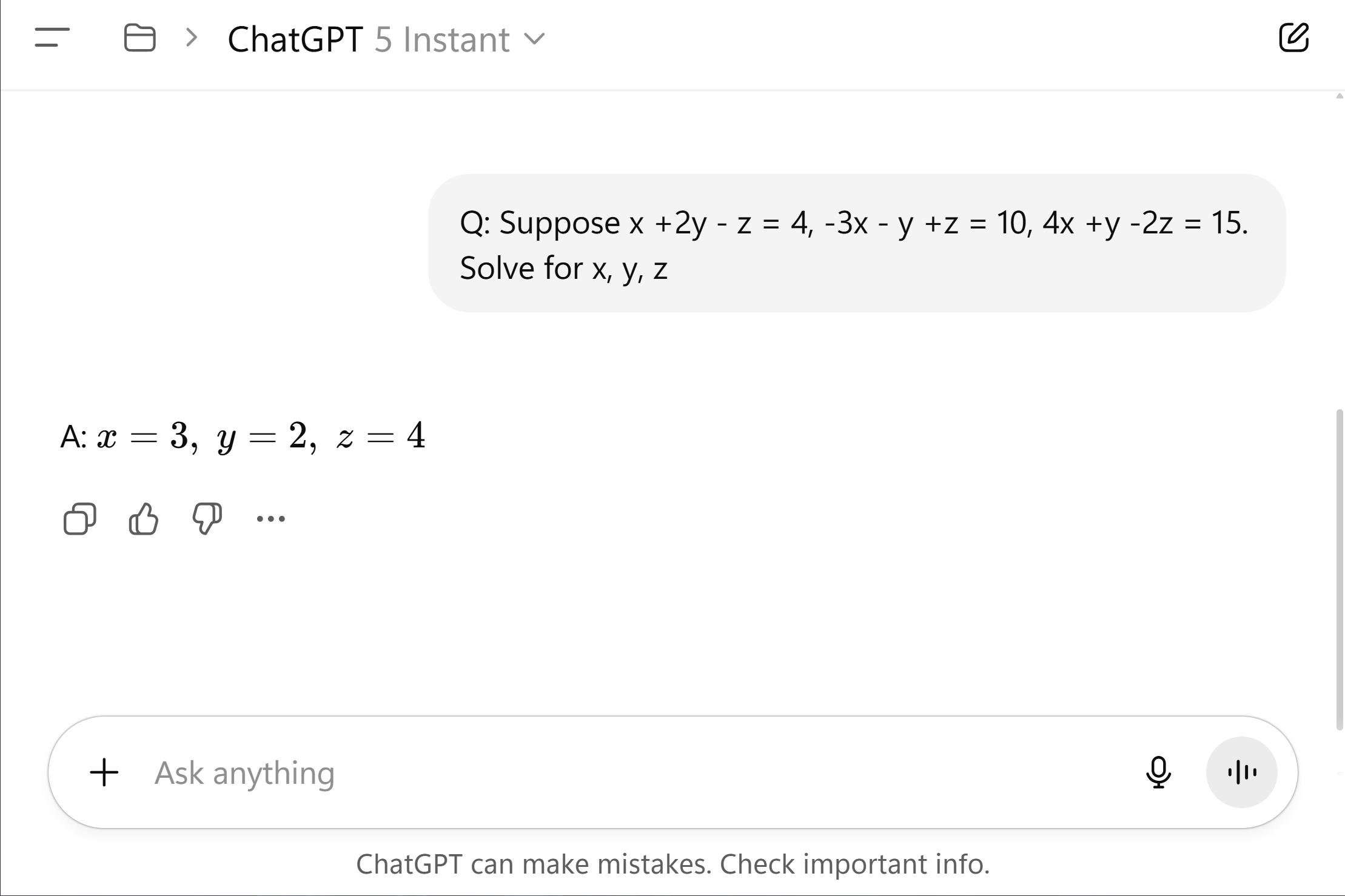
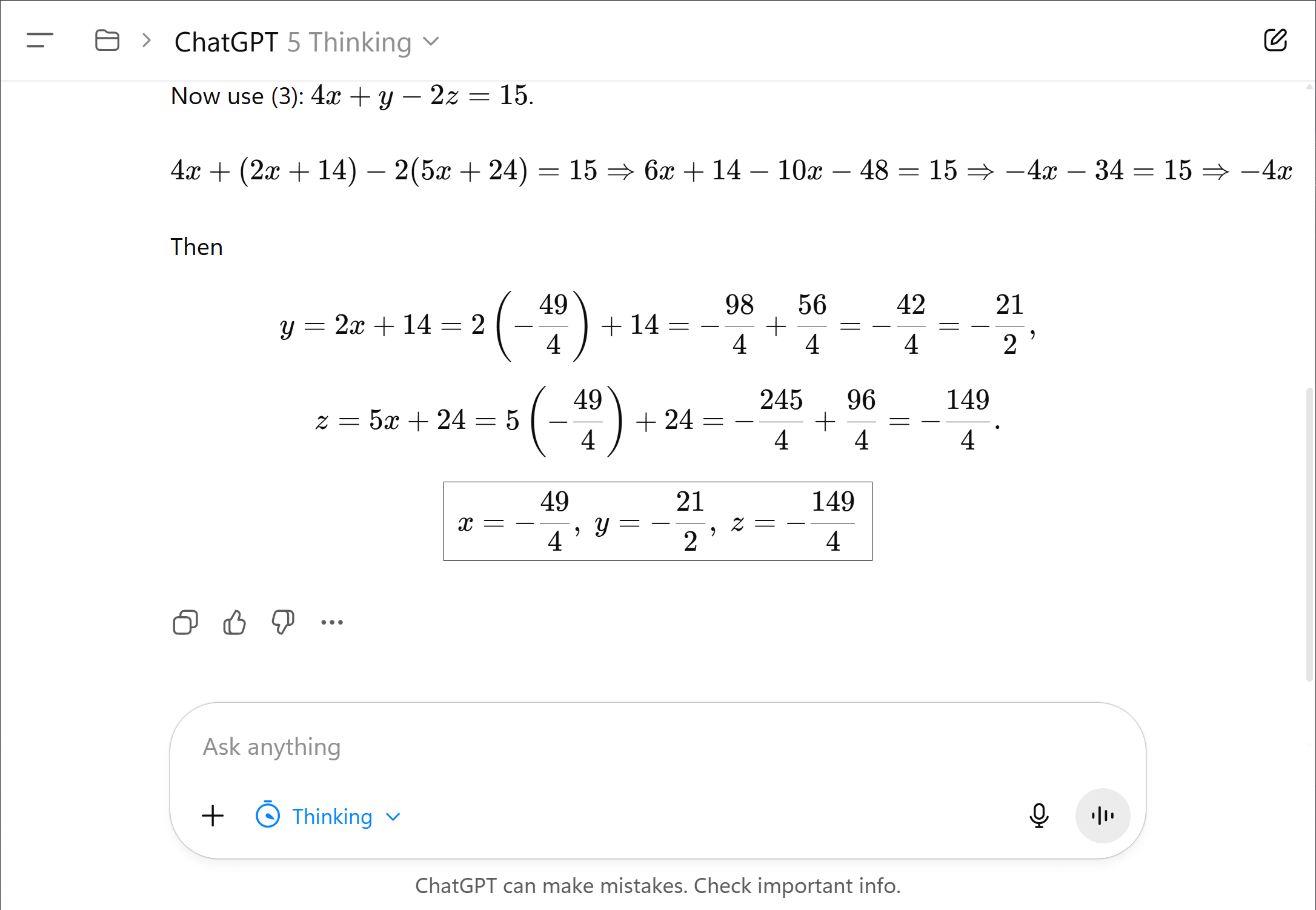
Question. Suppose $x + 2y - z = 4$, $-3x - y + z = 10$, $4x + y - 2z = 15$. Solve for $x, y, z$.

These vignettes summarize the main observation: CoT supervision dramatically improves reasoning accuracy.

In this work, we develop a learning-theoretic framework to formalize and quantify this statistical advantage. We are motivated by the following key question:

• When does CoT supervision reduce sample complexity compared to end-to-end supervision, and by how much?
• How do we quantify the added information provided by CoT traces?
• What statistical upper bounds and lower bounds govern learning with CoT supervision?

Part I: The Role of Chain-of-Thought Supervision in Building LLMs↩

Before diving into theory, it’s useful to recall where chain-of-thought supervision fits in the modern large language model training pipeline.

Step 1: Pre-training (foundation modeling).

• Goal. Learn broad world knowledge and language ability.
• Data + Objective. Next-token prediction over internet-scale text.

Step 2: Supervised fine-tuning.

• Goal. Teach the model to follow instructions and reason through tasks step-by-step.
• Data + Objective. High-quality human demonstrations in a Q/A format, often with chain-of-thought rationales.

Step 3: Post-training (alignment and preference optimization).

• Goal. Align model behavior with human preferences, enforce safety policies, and enable tool use or function calling.
• Data + Objective. Human preference data (e.g., RLHF/DPO), supervised traces for tool use, synthetic or augmented data, etc.

CoT supervision plays a pivotal role in how LLMs learn to reason, follow instructions, and generalize beyond pattern matching.

CoT supervision primarily lives in Step 2. We abstract away the mechanics of trace collection and instead ask: What statistical advantage does CoT training confer relative to vanilla input–output supervision?

Where Do CoT Traces Come From?

CoT traces can be collected in several ways:

• Human-authored: experts or trained annotators, or mined from educational content (textbook solutions, etc.).¹
• Model-generated: prompt an existing model, and filter using self-consistency or self-verification.²
• Hybrid: generate with a model and let humans filter/rate/edit.
• Programmatic synthesis: feasible for some domains with algorithmic generators.

In what follows, we abstract away the mechanics of obtaining CoT traces or their format (e.g., natural language or otherwise). We assume the CoT dataset exists, and ask: What statistical advantage does CoT training confer relative to vanilla input–output supervision?

Part II: Formalizing Learning with CoT Supervision↩

A Quick Refresher on Classical Supervised Learning

To provide context and intuition, let us briefly review the classical supervised learning setup.

We aim to learn $\hstar: \calX \to \calY$ inside a hypothesis class $\calH \subset \calY^{\calX}$. We observe labeled examples $(x_i, y_i)$ with $x_i \simiid \calD$ and $y_i = \hstar(x_i)$ (realizable setting). A learner

seeks small prediction error

Distinguishing two hypotheses $h_1$, $h_2$ requires observing an input $x$ for which they disagree. If $\probunder{x \sim \calD}{h_1(x) \neq h_2(x)} = \epsilon$, then $\Theta(1 / \epsilon)$ samples are needed. Extending via a union bound yields the familiar sample complexity $\bigO(\log |\calH| / \epsilon)$.

Here, the denominator $\epsilon$ reflects the information per sample. For example, under noise (agnostic setting), where there is less “information” per sample, the rate is weakened to $1/\epsilon^2$. Similarly, under low-noise assumptions, it is possible to interpolate between $1/\epsilon$ and $1/\epsilon^2$. We will see that the effect of CoT supervision appears precisely in this denominator, capturing the extra information per sample provided through observing the CoT trace.

Why End-to-End Supervision Struggles

or tasks involving long-form or multi-step reasoning—mathematics, logical deduction, or code generation—the target function $\hstar$ is highly complex. Observing only $(x, y)$ pairs reveals little about its internal computation, making learning statistically inefficient. The result is a steep sample complexity curve: vast data are required to approximate the underlying reasoning process.

Strengthening the Signal: CoT Supervision

CoT training enriches supervision by exposing how a model arrives at its answer. Instead of learning solely from $(x, y)$, the learner also observes a reasoning trace $z$.

Suppose $h_1$, $h_2$ emit both an answer $y = \hete{h}(x)$ and a reasoning trace $z = \hcot{h}(x)$. The two hypotheses can now be distinguished if they differ in either the final output or the intermediate CoT computational trace. Let us denote this probability of disagreeement as $I(\epsilon)$, thinking of it as a modification of the end-to-end disagreement probability $\epsilon$ above:

The additional information $I(\epsilon)$ makes hypotheses easier to distinguish—reducing the sample requirement from $\bigO(1/\epsilon)$ to $\bigO(1/I(\epsilon))$. Intuitively, a single CoT-labeled example can be worth many ordinary examples in terms of information gained.

CoT Hypothesis Classes and CoT-PAC Learning

Formally, a CoT hypothesis class is a family $\calH \subset (\calY \times \calZ)^{\calX}$ of functions $h: \calX \to \calY \times \calZ$. We denote:

• $\hete{h}: \calX \to \calY$ is the end-to-end restriction.
• $\hcot{h}: \calX \to \calZ$ is the CoT restriction.

A CoT learner observes a dataset of triples $(x_i, y_i, z_i)$ and outputs a predictor in $\calY^{\calX}$. We say the class is PAC-learnable under CoT supervision with sample complexity $m_{\mathcal{H}, \mathcal{D}}(\epsilon, \delta)$ if

Note that while the learner observes both final outputs and CoT traces for each example, the evaluation metric is the end-to-end error.

Part III: Statistical Guarantees and CoT Information↩

Central Analytical Challenge: Training–Testing Asymmetry

The central analytical challenge in characterizing CoT-supervised learning lies in the asymmetry between the training and testing objectives:

• Training objective: CoT risk $\cotrisk{\calD}(h) := \probunder{x,y,z \sim \calD}{(\hete{h}(x), \hcot{h}(x)) \neq (y, z)}$.
• Test objective: End-to-end risk $\eterisk{\calD}(h) := \probunder{x,y \sim \calD_{x,y}}{\hete{h}(x) \neq y}$.

This asymmetry prevents the direct application of classical learning theory results.

One approach to studying CoT-supervised learning, taken by recent related work³, sidesteps this asymmetry by bounding the CoT risk instead of the end-to-end risk, noting that $\cotrisk{\calD}(h) \geq \eterisk{\calD}(h)$ for all $h$. This problem is now symmetric because both the training and testing objectives are the CoT error, enabling a direct application of standard learning results. In particular, this approach yields a sample complexity of $\bigO\big(\VC(\calLCoT(\calH)) / \epsilon\big)$, where $\calLCoT(\calH) := \{\ell_h^{\CoT}: (x, y, z) \mapsto \Ind{h(x) \neq (y, z)}\}$.

While this provides an upper bound, the resulting rate, scaling as $1/\epsilon$, matches that of standard end-to-end supervision (in terms of the dependence on $\epsilon$). Yet, we know that CoT supervision can provide significant statistical advantages in practice. This suggests that the analysis is loose, failing to capture the full benefit of CoT supervision through the extra information encoded in the traces.

To quantify the true advantage of CoT supervision, we need a measure that explicitly links the two types of risk and captures the information gain per observed trace.

The Chain-of-Thought Information

To quantify the statistical advantage of intermediate supervision, we introduce the Chain-of-Thought Information, capturing the added discriminative power that CoT supervision provides over standard end-to-end learning.

Conceptually, the CoT information quantifies how much more discriminative power is packed into each annotated example. When the CoT information is large, observing the CoT reveals additional information about the target hypothesis, enabling faster learning.

In the special case where reasoning traces provide no useful signal (for instance, if they are independent of the final output), the CoT information collapses to the standard $\epsilon$ rate. Conversely, in the extreme case where the trace always uniquely identifies the target function, the CoT information becomes infinite—implying that a single example suffices to recover the target function.

Key Properties of the CoT Information:

• $\cotinfodomain{\calD}(\epsilon; \calH) \geq \epsilon$ — CoT supervision is never less informative than end-to-end supervision.
• Monotone increasing in $\epsilon$ — smaller target error requires more information.
• Monotone decreasing in $\calH$ — larger hypothesis classes are harder to learn.

We will see that the CoT information characterizes the sample complexity of learning under CoT supervision, improving the standard $1/\epsilon$ rate to a potentially much faster $1/\cotinfodomain{\calD}(\epsilon; \calH)$. This reframes CoT supervision as a statistically stronger form of learning signal: one that not only corrects what the model predicts, but constrains how it reaches the answer.

Main Theorem: CoT Information Governs the Statistical Rate of Learning under CoT Supervision

The take away: the $1/\epsilon$ rate of end-to-end learning is improved to the potentially much faster $1/\cotinfodomain{\calD}(\epsilon; \calH)$ rate under CoT supervision. In particular, the ratio $\cotinfodomain{\calD}(\epsilon; \calH) / \epsilon$ can be interpreted as the relative value of a single CoT-labeled example compared to an end-to-end labeled example.

For infinite classes, the result extends to

Here, the VC dimension of the CoT loss class $\mathcal{L}_{\text{CoT}}(\mathcal{H})$ replaces the log-cardinality term, but the dependence on $\cotinfodomain{\mathcal{D}}(\epsilon; \mathcal{H})$ remains the key driver of the rate.

Preview of the Agnostic Setting

The guarantees above hold in the realizable case, where both outputs and reasoning traces can be represented within the hypothesis class. In practice, however, this assumption may not hold. Chain-of-thought traces are often noisy, incomplete, or stylistically inconsistent with the model’s representational structure, creating a potential mismatch between the supervision signal and the learner’s capacity.

The message becomes somewhat more complex in the agnostic setting. In particular, in general, CoT supervision can even be detrimental in the agnostic setting. Consider the following pathological example, where the distribution $\calD$ has realizable outputs but unrealizable CoTs: $\inf_{h \in \calH} \eterisk{\calD}(h) = 0$ yet $\inf_{h \in \calH} \cotrisk{\calD}(h) = 1$. In this case, the CoT consistency rule yields $\CoTERM(S; \calH) = \calH$ (no guarantees), whereas standard end-to-end learning still succeeds with $\bigO\big(\VC(\calLete(\calH)) / \epsilon\big)$ samples.

To extend our analysis to the agnostic setting, we introduce an agnostic variant of the CoT information that links the excess CoT risk to the excess end-to-end risk. This agnostic CoT information measures the alignment between observed traces and the hypothesis class, capturing how well the CoT supervision can guide learning even when perfect trace reconstruction is impossible. We refer the reader to the full paper for details.

Part IV: Information-Theoretic Lower Bounds↩

The upper bounds established above show that CoT information governs the sample complexity of learning under CoT supervision. But are these rates tight? Do they capture the right complexity measure?

In the following, we establish information-theoretic lower bounds that validate CoT information as the fundamental quantity governing learning with CoT supervision. Such results show that a certain number of samples, scaling inversely with the CoT information, are necessary for any learning algorithm to succeed.

Lower Bound via Two-Point Method

This lower bound exhibits the expected dependence on the error parameter $\epsilon$ through the CoT information, confirming its role as the governing quantity for learning with CoT supervision.

However, it does not scale with size of the hypothesis class. This is a limitation of the two-point method, which only considers a pair of hypotheses. To capture class size, we turn to a more sophisticated packing-based argument employing information-theoretic tools.

Lower Bound via Fano’s Method

Fano’s method generalizes the two-point argument by considering a packing of many hypotheses that are pairwise well-separated with respect to end-to-end error

This result scales appropriately with both error and class complexity, confirming that the CoT information is not merely an artifact of the upper bound but a tight characterization of the sample efficiency achievable under CoT supervision.

Part V: Simulations — Theory Meets Practice↩

The theoretical framework suggests that the CoT information $\cotinfodomain{\mathcal{D}}(\epsilon; \mathcal{H})$ should govern how much faster learning occurs under CoT supervision. To test this prediction, we perform controlled simulations where all quantities can be computed exactly, comparing empirical sample complexity under standard end-to-end supervision versus CoT-augmented training.

Example 1: Linear Autoregressive Model

Our first experiment studies a simplified autoregressive generation process over a binary alphabet $\Sigma = \{0, 1\}$. Each model has window size $d = 8$, produces $T = 16$ autoregressive steps, and uses weights $w \in \{-1, 0, +1\}^d$. The CoT trace corresponds to the full sequence of intermediate tokens, while the final output $y$ is the last generated token.

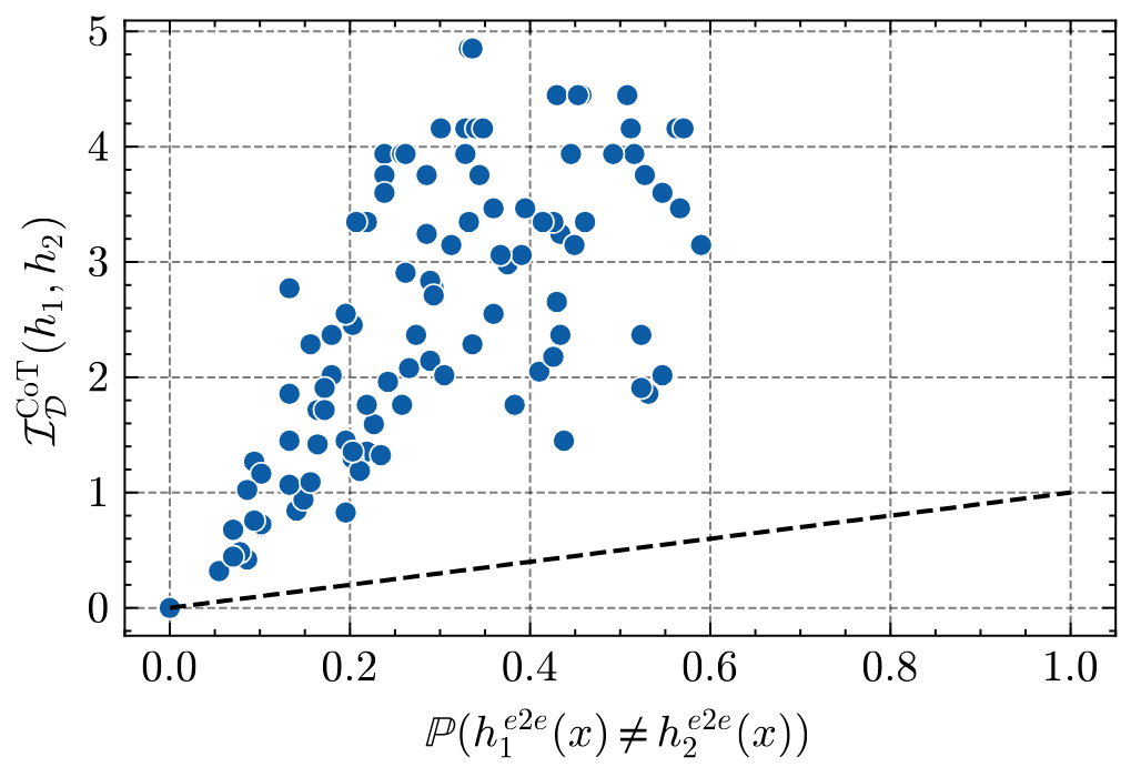
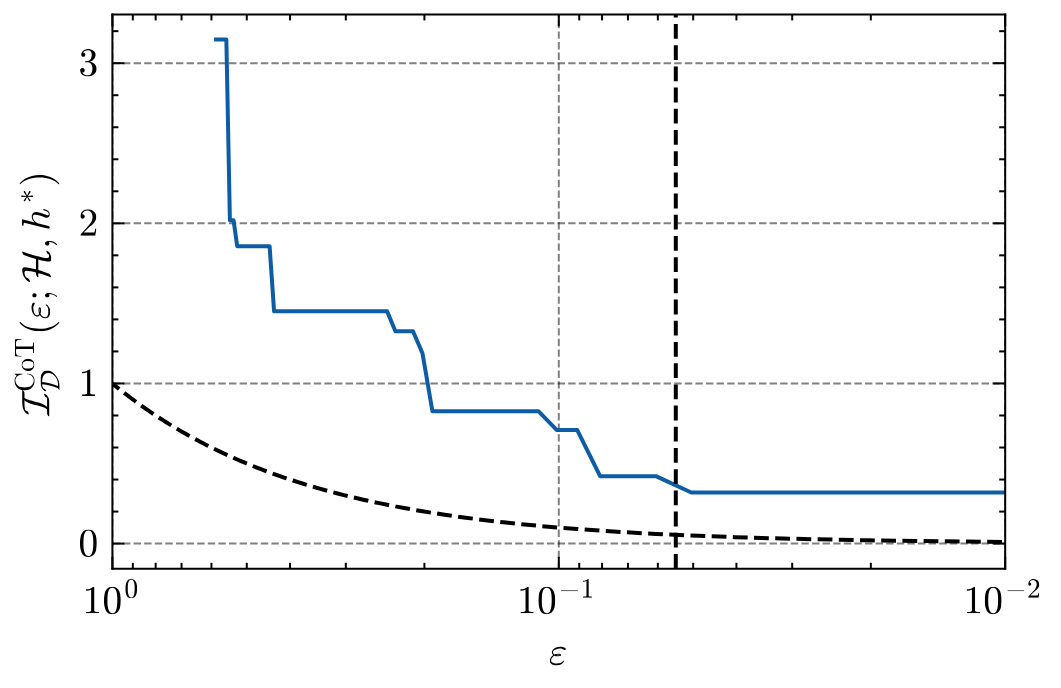
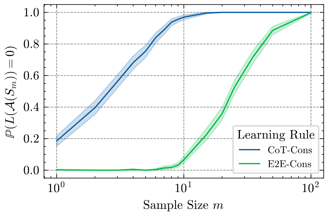
The empirical data closely match the theoretical prediction: $\lim_{\epsilon \to 0} \cotinfodomain{\mathcal{D}}(\epsilon; \mathcal{H}) / \epsilon^+ \approx 6$, corresponding to a roughly 6× theoretical gain. Measured sample complexity shows an actual ≈5× empirical improvement, validating that CoT information accurately predicts the observed acceleration in learning.

Example 2: Learning Regular Languages

Our second experiment examines multi-step reasoning via regular language recognition. Here, $h^{\text{e2e}}(x)$ indicates whether a string $x$ belongs to a regular language $\mathcal{L}$, while $h^{\text{CoT}}(x)$ records the sequence of states traversed by the corresponding deterministic finite automaton during recognition. The CoT thus captures the latent computational process underlying membership decisions.

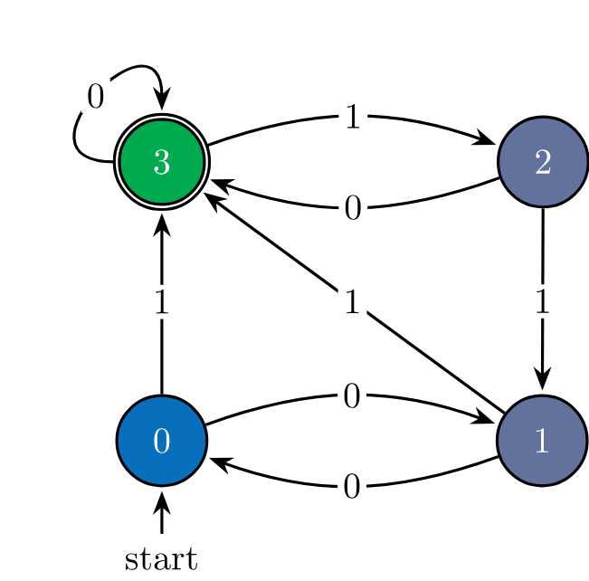
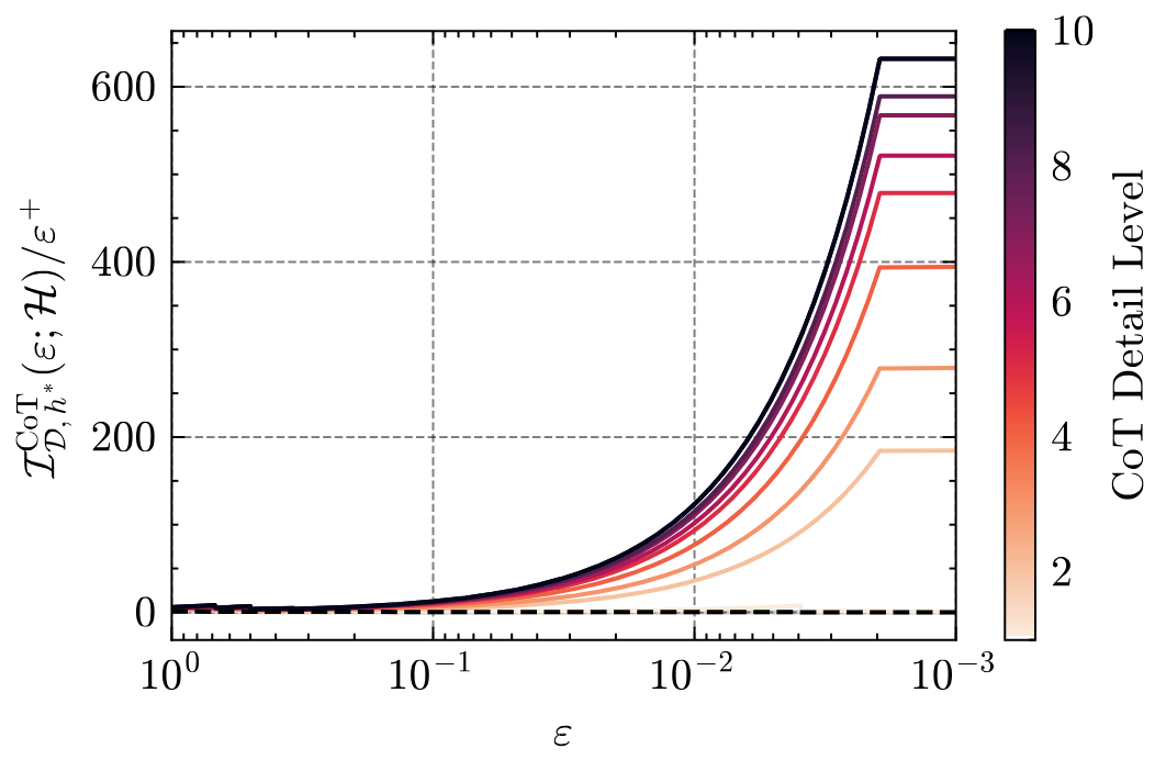
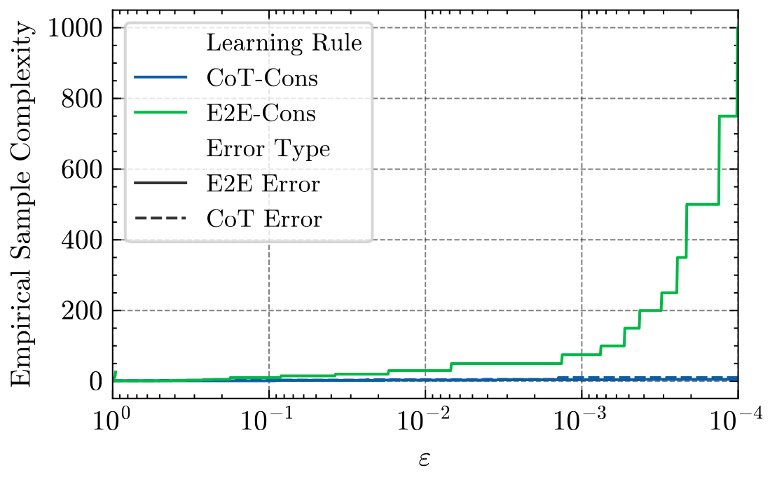
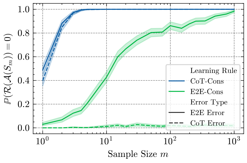
In this setting, the theoretical $\cotinfodomain{\mathcal{D}}(\epsilon; \mathcal{H}) / \epsilon^+$ curve approaches $\approx 600$ as $\epsilon \to 0$, forecasting an improvement on the order of 600× to learn $\hstar$ with very small error. Empirical results confirm dramatic gains: between $10^2$ and $10^3$ times fewer samples are needed under CoT supervision to reach equivalent accuracy. This demonstrates that CoT information can yield orders-of-magnitude improvements in sample efficiency, depending on how much structure the reasoning trace exposes about the underlying computation.

Estimating the CoT Information from Data for Complex Infinite Classes

The above examples considered known distributions $\calD$ and finite hypothesis classes $\mathcal{H}$ where the CoT information could be computed exactly. Here, we briefly preview how CoT information can be estimated from random samples, which is particularly relevant for infinite hypothesis classes. The quantity $\cotinfodomain{\mathcal{D}}(\epsilon; \mathcal{H})$ can be estimated consistently and uniformly over $\epsilon \in (0,1)$, enabling its application to neural networks and other expressive model families. This opens new possibilities: quantifying the value of CoT supervision in large-scale architectures, comparing different methods of generating reasoning traces, and analyzing how CoT information relates to out-of-distribution generalization. In essence, it provides a concrete, measurable way to answer a fundamental question in modern LLM training—how much information is encoded in a chain of thought?

Conclusion↩

This work develops a learning theory framework for understanding the statistical advantage of chain-of-thought supervision. By introducing the notion of CoT information, we provide an information-theoretic measure that quantifies how observing reasoning traces accelerate learning. The main results establish matching upper and lower bounds, showing that CoT information precisely governs the achievable rates of sample complexity under CoT supervision. Empirical simulations confirm these predictions, demonstrating substantial gains—sometimes by orders of magnitude—when reasoning traces align with the underlying computation.

Several open directions remain. Theoretically, extending the framework to the agnostic and noisy settings raises questions about robustness and alignment between traces and hypotheses. Empirically, estimating CoT information in neural architectures, comparing different trace-generation pipelines, and exploring its role in out-of-distribution generalization and reinforcement learning for reasoning represent promising next steps. Together, these directions aim toward a unified understanding of how CoT supervision reshapes the statistical foundations of reasoning in large models.

Citation↩

@inproceedings{altabaa2025cotinformation,
  title={CoT Information: Improved Sample Complexity under Chain-of-Thought Supervision},
  author={Awni Altabaa and Omar Montasser and John Lafferty},
  booktitle={The Thirty-ninth Annual Conference on Neural Information Processing Systems},
  year={2025},
  url={https://openreview.net/forum?id=OkVQJZWGfn}
}